Classifying protists into 155 (hierarchically organized) classes

An important component of my recent paper (previous post) on imaging protist (micro-eukaryotes) communities is a classifier that classifies each individual object into one of 155 classes. These classes are organized hierarchically, so that the first level corresponds to living/non-living object; then, if living, classifies it into phyla, and so on. This is the graphical representation we have in the paper:

Using a large training set (>18,000), we built a classifier capable of classifying objects into one these 155 classes with >82%.

What is the ML architecture we use? In the end, we use the traditional system: we compute many features and use a random forest trained on the full 155 classes. Why a random forest?

A random forest should be the first thing you try on a supervised classification problem (and perhaps also the last, lest you overfit). I did spent a few weeks trying different variations on this idea and none of them beat this simplest possible system. Random forests are also very fast to train (especially if you have a machine with many cores, as each tree can be learned independently).

As usual, the features were where the real work went. A reviewer astutely asked whether we really needed so many features (we compute 480 of them). The answer is yes. Even when selecting just the best features (which we wouldn’t know apriori, but let’s assume we had an oracle), it seems that we really do need a lot of features:

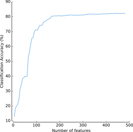
(This is Figure 3 — supplement 4: https://elifesciences.org/articles/26066/figures#fig3s4sdata1)

We need at least 200 features and it never really saturates. Furthermore, features are computed in groups (Haralick features, Zernike features, …), so we would not gain much

In terms of implementation, features were computed with mahotas (paper) and machine learning was done with scikit-learn (paper).

§

What about Deep Learning? Could we have used CNNs? Maybe, maybe not. We have a fair amount of data (>18,000 labeled samples), but some of the classes are not as well represented (in the pie chart above, the width of the classes represents how many objects are in the training set). A priori, it’s not clear it would have helped much.

Also, we may already be at the edge of what’s possible. Accuracy above 80% is already similar to human performance (unlike some of the more traditional computer vision problems, where humans perform with almost no mistakes and computers had very high error rates prior to the neural network revolution).
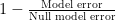
Evaluating Regression with Cross-Validation

I have been doing a bit of regression and have a few thoughts.

Most literature on regression comes from statisticians, not machine learning people. Perhaps for this reason, there is less emphasis on training/testing separation or cross-validation.

In particular, I have been thinking about how to get a general purpose measure of “how well can we predict this output.” Mean squared error \frac{1}{N} \sum (\hat{y}_i - y_i)^2,  where i is the cross-validated predictions for input i ) has some nice properties. However, it is meaningless as a number and it would be nice to normalize it.

What seems the most meaningful normalization is to use a null model which consists of outputting the mean of the training data. To make higher numbers be better, I first flip it around:

1 - \frac{ \sum (\hat{y}_i - y_i)^2 }{\sum (y_i - \bar{y})^2}

This is

1 - \frac{\text{Model error}}{\text{Null model error}}

The result can even be negative if the prediction is harmful. So, I actually want to use

N(\hat{y}, y) = \max \{ 1 - \frac{ \sum (\hat{y}_i - y_i)^2 }{\sum (y_i - \bar{y})^2}, 0 \}

This value is 0 for a meaningless prediction, 1 for a perfect one.

I am calling it N for normalized error reduction. In fact, I’ve tried looking and asking around for a literature name. So far, I have not found one.

§

In the case of a positive correlation with no bias, this reduces to the R-squared between  and y , also known to as the explained variance.

I like to look at the results in plots like this one

base

On the x-axis, I have the underlying output, and on the y-axis, the cross-validated (or out-of-bag prediction) for each sample. I also plot the diagonal. In this case, the prediction is very good and there is only a little noise pushing points away from the diagonal.

§

However, it does not reduce the R-squared in a few interesting cases:

  1. The model does not predict at all.

null

Let’s say that your output cannot be explained by the input at all. To simplify things, let’s assume you don’t even have an input, just a set of outputs, {y1..yN} , which you predict as the mean in the training set.

If you use leave-one-out-cross-validation (LOOCV), then this null-prediction has perfect (negative) correlation with the input (see also here and here! Its R-squared is 1!

If you are using LOOCV, then you’ll probably see this and catch it, but it might slip by if your using 10 folds and you don’t have a lot of data and accidently report it as low-but-significant (with 100 datapoints, and uniformly sampled yi , the R-squared is different from zero, with p-value < 0.05, 90% of the time! 25% of the times, the p-value is below 0.0001)

  1. Reversion to the mean models.

mean_regression

This is an instance of where your model was oversmoothed.

In this instance, your model predicts in the right direction, but it underpredicts. However, if you just report R-squared of the prediction, you’ll lead your readers to think you can predict very well.

It’s not always the case that you could just have gone back and multiplied all your coefficients by a number larger than 1. It may be that to get the larger coefficients would imply that you would get noise in the output. This would not happen in traditional regression problems, but in p > n settings, where penalized regression is necessary, it can and does happen (maybe it is an indication to try relaxed lasso).

  1. Biased models

biased

If your models are biased, this naturally introduces a penalty. R-squared is invariant to addition (R2( + B, y) =  R2(, y) ), but N is not. In fact, if the correlation is positive,

R2(\hat{y}, y) = \max_B N(\hat{y} + B, y).

I most often see this when comparing human annotations. People have very similar trends, but one of the operators will consistenly report a lower value.

In some cases this may not matter and in others it will (if Matt always needs to give a bigger discount than John to get a sale, this does not mean that Matt and John are equivalent salesman).

§

In all of these, the R-squared is excellent, but I think it is overselling how good the prediction is, whilst N is more honest.

FAQ: How Many Clusters Did You Use?

Luis Pedro Coelho, Joshua D. Kangas, Armaghan Naik, Elvira Osuna-Highley, Estelle Glory-Afshar, Margaret Fuhrman, Ramanuja Simha, Peter B. Berget, Jonathan W. Jarvik, and Robert F. Murphy, Determining the subcellular location of new proteins from microscope images using local features in Bioinformatics, 2013 [Advanced Access]  [Previous discussion on this blog]

Coelho, Luis Pedro, Tao Peng, and Robert F. Murphy. “Quantifying the Distribution of Probes Between Subcellular Locations Using Unsupervised Pattern Unmixing.” Bioinformatics 26.12 (2010): i7–i12. DOI: 10.1093/bioinformatics/btq220  [Previous discussion on this blog]

Both of my Bioinformatics papers above use the concept of bag of visual words. The first for classification, the second for pattern unmixing.

Visual words are formed by clustering local appearance descriptors. The descriptors may have different origins (see the papers above and the references below) and the visual words are used differently, but the clustering is a common intermediate step.

A common question when I present this work is how many clusters do I use? Here’s the answer: it does not matter too much.

I used to just pick a round number like 256 or 512, but for the local features paper, I decided to look at the issue a bit closer. This is one of the panels from the paper, showing accuracy (y-axis) as a function of the number of clusters (x-axis):

profile-field-dna+-RT-widefield-gs

As you can see, if you use enough clusters, you’ll do fine. If I had extended the results rightwards, then you’d see a plateau (read the full paper & supplements for these results) and then a drop-off. The vertical line shows N/4, where N is the number of images in the study. This seems like a good heuristic across several datasets.

One very interesting result is that choosing clusters by minimising AIC can be counter-productive! Here is the killer data (remember, we would be minimizing the AIC):

accuracy-aic-rt-widefield-gs

Minimizing the AIC leads to lower accuracy! AIC was never intended to be used in this context, of course, but it is often used as a criterion to select the number of clusters. I’ve done it myself.

Punchline: If doing classification using visual words, minimsing AIC may be detrimental, try using N/4 (N=nr of images).

Other References

This paper (reviewed before on this blog) presents supporting data too:

Noa Liscovitch, Uri Shalit, & Gal Chechik (2013). FuncISH: learning a functional representation of neural ISH images Bioinformatics DOI: 10.1093/bioinformatics/btt207

Old Work: Unsupervised Subcellular Pattern Unmixing

Continuing down nostalgia lane, here is another old paper of mine:

Coelho, Luis Pedro, Tao Peng, and Robert F. Murphy. “Quantifying the Distribution of Probes Between Subcellular Locations Using Unsupervised Pattern Unmixing.” Bioinformatics 26.12 (2010): i7–i12. DOI: 10.1093/bioinformatics/btq220

I have already discussed the subcellular location determination problem. This is Given images of a protein, can we assign it to an organelle?

This is, however, a simplified version of the world: many proteins are present in multiple organelles. They may move between organelles in response to a stimulus or as part of the cell cycle. For example, here is an image of mitochondria in green (nuclei in red):

img17

Here is one of lysosomes:

img71

And here is a mix of both!:

img77-2

This is a dataset constructed for the purpose of this work, so we know what is happening, but it simulates the situation where a protein is present in two locations simultaneously.

Thus, we can move beyond simple assignment of a protein to an organelle to assigning it to multiple organelles. In fact, some work (both from the Murphy group and others) has looked at subcellular location classification using multiple labels per image. This, however, is still not enough: we want to quantify this.

This is the pattern unmixing problem. The goal is to go from an image (or a set of images) to something like the following: This is 30% nuclear and 70% cytoplasmic, which is very different from 70% nuclear and 30% cytoplasmic. The basic organelles can serve as the base patterns [1].

Before our paper, there was some work in approaching this problem from a supervised perspective: Given examples of different organelles (ie, of markers that locate to a single organelle), can we automatically build a system which when given images of a protein which is distributed in multiple organelles, can figure out which fraction comes from each organelle?

Our paper extended this to work to the unsupervised case: can you learn a mixture when you do not know which are the basic patterns?

References

Determining the distribution of probes between different subcellular locations through automated unmixing of subcellular patterns Tao Peng, Ghislain M. C. Bonamy, Estelle Glory-Afshar, Daniel R. Rines, Sumit K. Chanda, and Robert F. Murphy PNAS 2010 107 (7) 2944-2949; published ahead of print February 1, 2010, doi:10.1073/pnas.0912090107

Object type recognition for automated analysis of protein subcellular location T Zhao, M Velliste, MV Boland, RF Murphy Image Processing, IEEE Transactions on 14 (9), 1351-1359

[1] This is still a limited model because we are not sure even how many base patterns we should consider, but it will do for now.

Old papers: Structured Literature Image Finder (SLIF)

Still going down memory lane, I am presenting a couple of papers:

Structured literature image finder: extracting information from text and images in biomedical literature LP Coelho, A Ahmed, A Arnold, J Kangas, AS Sheikh, EP Xing, WW Cohen, RF Murphy Linking Literature, Information, and Knowledge for Biology, 23-32 [DOI] [Murphylab PDF]

Structured literature image finder: Parsing text and figures in biomedical literature A Ahmed, A Arnold, LP Coelho, J Kangas, AS Sheikh, E Xing, W Cohen, RF Murphy Web Semantics: Science, Services and Agents on the World Wide Web 8 (2), 151-154 [DOI]

These papers refer to SLIF, which was the Subcellular Location Image Finder and later the Structured Literature Image Finder.

The initial goals of this project were to develop a system which parsed the scientific literature and extracted figures (including the caption). Using text-processing, the system attempted to guess what the image depicted and using computer vision, the system attempted to interpret the image.

In particular, the focus was on subcellular image analysis for different proteins from fluorescent micrographs in published literature.

slif-overview

§

Additionally, there was a topic-model based navigation based on both images and the caption-text. This allowed for latent model based navigation. Unfortunately, the site is currently offline, but our user-study showed that it was a meaningful navigation model.

§

The final result was a proof-of-concept system. Most of the subsystems worked at reasonably high accuracy, but it was not sufficient for the overall inferrences to be of very high accuracy (if there are six steps in an inferene step and each has 90% accuracy, then you are just about 50/50, which is much better than random guessing in large inference spaces, but still not directly trustable).

I think the vision is still valid and eventually the technology will be good enough. There is a lot of information inside the biological literature which is not always so obvious to get at and that much of this is in the form of image. SLIF was a first stab at getting at this data in addition to the text-based approaches that are more well known.

§

More information about SLIF (including references to the initial SLIF papers, of which I was not a part).

The False Hope of Usable Data Analysis

I changed the regular schedule of the posts because I wanted to write down these ideas.

A few days ago, in a panel at EuBIAS, I argued again that scientists should learn how to programme. I also argued that usability of bioimage analysis was a false hope.

Now, to be sure: usability is great, but usability does not mean usable without programming skills. Good usable programming environments can be the most usable way to achieve something[1]. I find the Python environment one of the most usable for data analysis currently, although there is still a lot of work which could improve it.

§

road_signs

We can build communication systems without words, but only if the vocabulary is very limited. Otherwise, people need to learn how to read [2]. I think this a good analogy for non-programming environments.

§

The problem is that image analysis (or data analysis) is not a closed goal. Whatever we are doing today, will probably be packaged into simple-to-use tools, but the problems will grow in size and complexity.

For a fixed target, like sending email or writing a blog, we can build nice tools that don’t require programming. Any modern email client basically does email well enough. There is probably only a small set of behaviours we want our blogs to do (like scheduling a post) and I think we can get a small set of features that covers 95%+ of uses. There might be a need for a few hundred plugins, but not constant innovation. There is no constant pressure to do 10 times more.

But data analysis is not in the same category as sending email. It’s an open-ended problem, which will grow continuously, which has been growing continuously. Only a full-blown artificial intelligence system will be able to deal with the sort of analyses that we will want to do in 10 years. There are even analyses that we already want to do, but do not yet have the right code and tools.

§

If anything, as time has passed, I have felt more and more of a need to think in low-level terms [3].

A few years ago, push-button analysis was sufficient for most problems. Load your data into Excel, select the rows, and plot. Fit a line, compute some stats. STATA gave you a bit more power if Excel did not suffice. Now, the problems grew and push-button solutions do not scale. Not only do we have more data, we have more complex, more unstructured data.

Afew years ago, pointing out that Excel can only handle 1 million rows would have made you seem like a technically-obsessed weirdo, now it is a serious limitation.

A few years ago, people were writing things like feel free to use interpreted languages, it doesn’t matter that you’re losing performance compared to C; computers are super-fast, waste them. Now, there is much more interest in building implementations that are as fast as C (normally using Just-in-time compilation).

This will not get better and just saying that tools should be easier for non-programmers is missing the point.

§

Programming is like writing: a general purpose technological skill which transforms all activities. And this means that, eventually, it becomes useful (or even necessary) for many activities which are outside the core of programming (who’d have thought a salesperson would have to know how to read and write? A firefighter?).

Almost any job that does not require programming is one which can be done by a robot. Except entertainment and those jobs that Tyler Cowen, for lack of a better word, calls marketing. Tyler calls them marketing, but prostitution might be just as accurate, as it is about providing not a specific service or product, which could be provided by a machine, but the general positive feeling that comes from human contact [4].

Related

Bayes and Big Data by Cosma Shalizi

The Average is Over by Tyler Cowen

[1] If you wish, read scripting for programming. I never cared much for this division.
[2] If you google for traffic signs you’ll see that actually most images have at least one sign with words or images.
[3] The need to managing parallelism (as our cores multiply, but not get faster) and memory access patterns as data grows faster than RAM have forced me to think about exactly what is happening in my machines.
[4] Obviously, Tyler is right to use the word marketing even if it’s not a good fit. Prostitution has a strong negative charge..

Is Cell Segmentation Needed for Cell Analysis?

Having just spent some posts discussing a paper on nuclear segmentation (all tagged posts), let me ask the question:

Is cell segmentation needed? Is this a necessary step in an analysis pipeline dealing with fluorescent cell images?

This is a common FAQ whenever I give a talk on my work which does not use segmentation, for example, using local features for classification (see the video). It is a FAQ because, for many people, it seems obvious that the answer is that Yes, you need cell segmentation. So, when they see me skip that step, they ask: shouldn’t you have segmented the cell regions?

Here is my answer:

Remember Vapnik‘s dictum [1]do not solve, as an intermediate step, a harder problem than the problem you really need to solve.

Thus the question becomes: is your scientific problem dependent on cell segmentation? In the case, for example, of subcellular location determination, it is not: all the cells in the same field display the same phenotype, your goal being the find out what it is. Therefore, you do not need to have an answer for each cell, only for the whole field.

In other problems, you may need to have a per-cell answer: for example in some kinds of RNAi experiment only a fraction of the cells in a field display the RNAi phenotype and the others did not take up the RNAi. Therefore, segmentation may be necessary. Similarly, if a measurement such as distance of fluorescent bodies to cell membrane is meaningful, by itself (as opposed to being used as a feature for classification), then you need segmentation.

However, sometimes you can get away without segmentation.

§

An important point to note is the following: while it may be good to have access to perfect classification, imperfect classification (i.e., the type you actually get), may not help as much as the perfect kind.

§

Just to be sure, I was not the first person to notice that you do not need segmentation for subcellular location determination. I think this is the first reference:

Huang, Kai, and Robert F. Murphy. “Automated classification of subcellular patterns in multicell images without segmentation into single cells.” Biomedical Imaging: Nano to Macro, 2004. IEEE International Symposium on. IEEE, 2004. [Google scholar link]

[1] I’m quoting from memory. It may a bit off. It sounds obvious when you put it this way, but it is still often not respected in practice.